[1]:
%matplotlib inline
Linear Least-Squares Inversion with Tikhonov Regularization
Here we demonstrate the basics of inverting data with SimPEG by considering a linear inverse problem. We formulate the inverse problem as a least-squares optimization problem. For this tutorial, we focus on the following:
- Defining the forward problem
- Defining the inverse problem (data misfit, regularization, optimization)
- Specifying directives for the inversion
- Recovering a set of model parameters which explains the observations
Import Modules
[1]:
import numpy as np
import matplotlib.pyplot as plt

from discretize import TensorMesh

from SimPEG import (
    simulation,
    maps,
    data_misfit,
    directives,
    optimization,
    regularization,
    inverse_problem,
    inversion,
)

# sphinx_gallery_thumbnail_number = 3
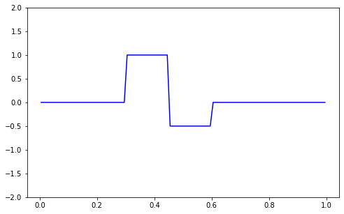
Defining the Model and Mapping
Here we generate a synthetic model and a mappig which goes from the model space to the row space of our linear operator.
[2]:
nParam = 100  # Number of model paramters

# A 1D mesh is used to define the row-space of the linear operator.
mesh = TensorMesh([nParam])

# Creating the true model
true_model = np.zeros(mesh.nC)
true_model[mesh.vectorCCx > 0.3] = 1.0
true_model[mesh.vectorCCx > 0.45] = -0.5
true_model[mesh.vectorCCx > 0.6] = 0

# Mapping from the model space to the row space of the linear operator
model_map = maps.IdentityMap(mesh)

# Plotting the true model
fig = plt.figure(figsize=(8, 5))
ax = fig.add_subplot(111)
ax.plot(mesh.vectorCCx, true_model, "b-")
ax.set_ylim([-2, 2])
[2]:
(-2.0, 2.0)
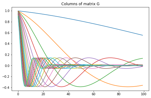
Defining the Linear Operator
Here we define the linear operator with dimensions (nData, nParam). In practive, you may have a problem-specific linear operator which you would like to construct or load here.
[3]:
# Number of data observations (rows)
nData = 20

# Create the linear operator for the tutorial. The columns of the linear operator
# represents a set of decaying and oscillating functions.
jk = np.linspace(1.0, 60.0, nData)
p = -0.25
q = 0.25


def g(k):
    return np.exp(p * jk[k] * mesh.vectorCCx) * np.cos(
        np.pi * q * jk[k] * mesh.vectorCCx
    )


G = np.empty((nData, nParam))

for i in range(nData):
    G[i, :] = g(i)

# Plot the columns of G
fig = plt.figure(figsize=(8, 5))
ax = fig.add_subplot(111)
for i in range(G.shape[0]):
    ax.plot(G[i, :])

ax.set_title("Columns of matrix G")
[3]:
Text(0.5, 1.0, 'Columns of matrix G')
Defining the Simulation
The simulation defines the relationship between the model parameters and predicted data.
[4]:
sim = simulation.LinearSimulation(mesh, G=G, model_map=model_map)
c:\users\u0102388\pyprojects\wavelet-based-inversion\venv\lib\site-packages\SimPEG\simulation.py:547: UserWarning: G has not been implemented for the simulation
  warnings.warn("G has not been implemented for the simulation")
Predict Synthetic Data
Here, we use the true model to create synthetic data which we will subsequently invert.
[5]:
# Standard deviation of Gaussian noise being added
std = 0.01
np.random.seed(1)

# Create a SimPEG data object
data_obj = sim.make_synthetic_data(true_model, relative_error=std, add_noise=True)
Define the Inverse Problem
The inverse problem is defined by 3 things:
1) Data Misfit: a measure of how well our recovered model explains the field data
2) Regularization: constraints placed on the recovered model and a priori information
3) Optimization: the numerical approach used to solve the inverse problem
[6]:
# Define the data misfit. Here the data misfit is the L2 norm of the weighted
# residual between the observed data and the data predicted for a given model.
# Within the data misfit, the residual between predicted and observed data are
# normalized by the data's standard deviation.
dmis = data_misfit.L2DataMisfit(simulation=sim, data=data_obj)

# Define the regularization (model objective function).
reg = regularization.Tikhonov(mesh, alpha_s=1.0, alpha_x=1.0)

# Define how the optimization problem is solved.
opt = optimization.InexactGaussNewton(maxIter=50)

# Here we define the inverse problem that is to be solved
inv_prob = inverse_problem.BaseInvProblem(dmis, reg, opt)
Define Inversion Directives
Here we define any directiveas that are carried out during the inversion. This includes the cooling schedule for the trade-off parameter (beta), stopping criteria for the inversion and saving inversion results at each iteration.
[7]:
# Defining a starting value for the trade-off parameter (beta) between the data
# misfit and the regularization.
starting_beta = directives.BetaEstimate_ByEig(beta0_ratio=1e-4)

# Setting a stopping criteria for the inversion.
target_misfit = directives.TargetMisfit()

# The directives are defined as a list.
directives_list = [starting_beta, target_misfit]
Setting a Starting Model and Running the Inversion
To define the inversion object, we need to define the inversion problem and the set of directives. We can then run the inversion.
[8]:
# Here we combine the inverse problem and the set of directives
inv = inversion.BaseInversion(inv_prob, directives_list)

# Starting model
starting_model = np.zeros(nParam)

# Run inversion
recovered_model = inv.run(starting_model)
SimPEG.InvProblem will set Regularization.mref to m0.

        SimPEG.InvProblem is setting bfgsH0 to the inverse of the eval2Deriv.
        ***Done using same Solver and solverOpts as the problem***
model has any nan: 0
============================ Inexact Gauss Newton ============================
  #     beta     phi_d     phi_m       f      |proj(x-g)-x|  LS    Comment
-----------------------------------------------------------------------------
x0 has any nan: 0
   0  1.86e+02  1.00e+05  0.00e+00  1.00e+05    1.26e+06      0
   1  1.86e+02  4.68e+04  3.50e-01  4.68e+04    8.00e+04      0
   2  1.86e+02  3.18e+04  1.35e+00  3.21e+04    5.90e+04      0
   3  1.86e+02  1.75e+04  5.21e+00  1.85e+04    5.36e+04      0   Skip BFGS
   4  1.86e+02  1.16e+04  5.18e+00  1.25e+04    8.12e+04      0
   5  1.86e+02  8.05e+03  8.09e+00  9.55e+03    4.44e+04      0
   6  1.86e+02  4.39e+03  1.19e+01  6.59e+03    5.39e+04      0
   7  1.86e+02  3.33e+03  1.24e+01  5.65e+03    2.83e+04      0
   8  1.86e+02  2.87e+03  1.31e+01  5.30e+03    8.05e+04      0
   9  1.86e+02  2.38e+03  1.38e+01  4.95e+03    3.99e+04      0
  10  1.86e+02  1.60e+03  1.55e+01  4.48e+03    6.49e+04      0
  11  1.86e+02  1.32e+03  1.64e+01  4.37e+03    6.36e+04      0
  12  1.86e+02  1.19e+03  1.66e+01  4.28e+03    4.79e+04      0
  13  1.86e+02  1.15e+03  1.65e+01  4.22e+03    6.65e+04      0
  14  1.86e+02  7.66e+02  1.72e+01  3.97e+03    8.01e+03      0   Skip BFGS
  15  1.86e+02  6.29e+02  1.76e+01  3.91e+03    2.86e+04      0
  16  1.86e+02  5.57e+02  1.76e+01  3.83e+03    2.20e+04      0   Skip BFGS
  17  1.86e+02  5.61e+02  1.74e+01  3.81e+03    1.74e+04      0
  18  1.86e+02  6.09e+02  1.71e+01  3.79e+03    1.76e+04      0   Skip BFGS
  19  1.86e+02  6.08e+02  1.71e+01  3.79e+03    1.38e+04      0
  20  1.86e+02  6.44e+02  1.68e+01  3.77e+03    1.66e+04      0   Skip BFGS
  21  1.86e+02  6.14e+02  1.69e+01  3.77e+03    1.38e+04      0
  22  1.86e+02  6.11e+02  1.69e+01  3.76e+03    1.32e+04      0   Skip BFGS
  23  1.86e+02  5.91e+02  1.70e+01  3.76e+03    1.97e+04      0
  24  1.86e+02  5.43e+02  1.72e+01  3.75e+03    2.16e+04      0   Skip BFGS
  25  1.86e+02  5.54e+02  1.72e+01  3.75e+03    1.51e+04      0
  26  1.86e+02  5.71e+02  1.71e+01  3.75e+03    1.48e+04      0   Skip BFGS
  27  1.86e+02  5.61e+02  1.71e+01  3.75e+03    1.47e+04      0
  28  1.86e+02  5.60e+02  1.71e+01  3.75e+03    1.48e+04      0   Skip BFGS
  29  1.86e+02  5.61e+02  1.71e+01  3.75e+03    1.49e+04      0
  30  1.86e+02  5.55e+02  1.71e+01  3.74e+03    1.40e+04      0   Skip BFGS
  31  1.86e+02  5.55e+02  1.71e+01  3.74e+03    1.41e+04      0
  32  1.86e+02  5.42e+02  1.71e+01  3.72e+03    1.03e+04      0   Skip BFGS
  33  1.86e+02  5.42e+02  1.71e+01  3.72e+03    1.03e+04      0
  34  1.86e+02  5.30e+02  1.71e+01  3.72e+03    8.23e+03      0
  35  1.86e+02  5.01e+02  1.73e+01  3.71e+03    4.98e+03      0   Skip BFGS
  36  1.86e+02  5.11e+02  1.72e+01  3.71e+03    4.00e+03      0
  37  1.86e+02  5.07e+02  1.72e+01  3.71e+03    2.92e+03      0
  38  1.86e+02  5.13e+02  1.72e+01  3.71e+03    5.65e+03      0   Skip BFGS
  39  1.86e+02  5.10e+02  1.72e+01  3.71e+03    5.97e+02      0
  40  1.86e+02  5.12e+02  1.72e+01  3.71e+03    1.73e+03      0   Skip BFGS
  41  1.86e+02  5.14e+02  1.72e+01  3.71e+03    1.68e+03      0
  42  1.86e+02  5.13e+02  1.72e+01  3.71e+03    1.37e+03      0
  43  1.86e+02  5.12e+02  1.72e+01  3.71e+03    2.83e+03      0
  44  1.86e+02  5.14e+02  1.72e+01  3.71e+03    1.50e+03      0   Skip BFGS
  45  1.86e+02  5.16e+02  1.72e+01  3.71e+03    1.71e+03      0
  46  1.86e+02  5.16e+02  1.72e+01  3.71e+03    1.83e+03      0   Skip BFGS
  47  1.86e+02  5.16e+02  1.72e+01  3.71e+03    1.71e+03      0
  48  1.86e+02  5.13e+02  1.72e+01  3.71e+03    1.78e+03      0   Skip BFGS
  49  1.86e+02  5.13e+02  1.72e+01  3.71e+03    1.83e+03      0
  50  1.86e+02  5.13e+02  1.72e+01  3.71e+03    1.67e+03      0
------------------------- STOP! -------------------------
1 : |fc-fOld| = 4.0445e-04 <= tolF*(1+|f0|) = 1.0000e+04
1 : |xc-x_last| = 5.0070e-04 <= tolX*(1+|x0|) = 1.0000e-01
0 : |proj(x-g)-x|    = 1.6708e+03 <= tolG          = 1.0000e-01
0 : |proj(x-g)-x|    = 1.6708e+03 <= 1e3*eps       = 1.0000e-02
1 : maxIter   =      50    <= iter          =     50
------------------------- DONE! -------------------------
[ ]:
Plotting Results
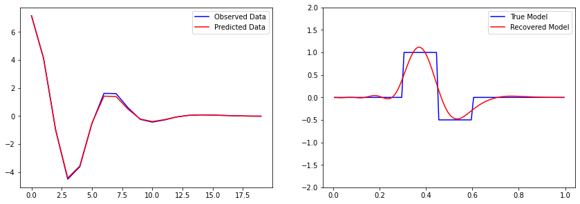
[9]:
# Observed versus predicted data
fig, ax = plt.subplots(1, 2, figsize=(12 * 1.2, 4 * 1.2))
ax[0].plot(data_obj.dobs, "b-")
ax[0].plot(inv_prob.dpred, "r-")
ax[0].legend(("Observed Data", "Predicted Data"))

# True versus recovered model
ax[1].plot(mesh.vectorCCx, true_model, "b-")
ax[1].plot(mesh.vectorCCx, recovered_model, "r-")
ax[1].legend(("True Model", "Recovered Model"))
ax[1].set_ylim([-2, 2])
[9]:
(-2.0, 2.0)